Simplifying Data with PCA and t-SNE — The Dynamic Duo of Dimensionality Reduction!

Thumbnail Created via Canva

We use Python for a variety of purposes in data science, including for machine learning and data visualization. One area where Python excels is in its ability to handle large amounts of data. However, this abundance of data can sometimes lead to a problem known as the “curse of dimensionality.” In these cases, it can be helpful to use dimensionality reduction techniques to simplify the data and make it easier to work with.

What exactly is Dimensionality reduction?

Dimensionality reduction is the process of taking high-dimensional data and reducing it down to a lower number of dimensions, usually 2 or 3, for the purpose of visualization or to make it easier to work with. By doing this, you can often uncover hidden patterns in the data that might have been missed otherwise.

In addition to helping to uncover patterns in data, dimensionality reduction can also improve the performance of machine learning algorithms. For example, reducing the number of features in a dataset can make it easier and faster for a machine learning algorithm to learn and make predictions.

Overall, dimensionality reduction is a powerful tool in the data scientist’s arsenal. By simplifying complex data, it can help you gain better insights and make more informed decisions. Whether you’re working on a machine learning project or just trying to make sense of a large dataset, it’s definitely worth exploring dimensionality reduction techniques.

In this article, we’ll be exploring two popular dimensionality reduction techniques: PCA (Principal Component Analysis) and t-SNE (t-Distributed Stochastic Neighbor Embedding). Both of these techniques are widely used in data science and have proven to be effective in reducing the dimensionality of data.

Python Libraries

Libraries used:

Python Libraries To perform dimensionality reduction in Python, we’ll be using Scikit-learn library:

Scikit-learn: This library provides a wide range of machine learning algorithms, including PCA and t-SNE.

Matplotlib: This library is used for data visualization, and we’ll be using it to create visual representations of the data after it has been reduced in dimensionality.

Let’s dive into the code!

PCA

Our first task is to import the libraries we’ll be using:

import numpy as np
import matplotlib.pyplot as plt
from sklearn.decomposition import PCA

Next, we’ll load some sample data using the load_digits function from the sklearn.datasets module:

from sklearn.datasets import load_digits
digits = load_digits()

Now we can create a PCA object and fit our data to it:

pca = PCA(n_components=2)
reduced_data = pca.fit_transform(digits.data)

Here, we’ve specified that we want to reduce the data down to two dimensions using the n_components parameter. We can then use the fit_transform method to fit the data to the PCA object and transform it into its reduced form.

Finally, we’ll use the scatter function from matplotlib to create a scatter plot of the reduced data:

plt.scatter(reduced_data[:, 0], reduced_data[:, 1], c=digits.target)
plt.show()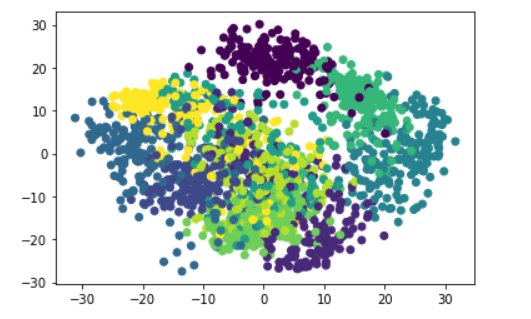

Scatterplot

t-SNE

The process for using t-SNE is similar to that of PCA. First, we import the necessary libraries:

import numpy as np
import matplotlib.pyplot as plt
from sklearn.manifold import TSNE

Next, we load some sample data in the same way as before:

from sklearn.datasets import load_digits
digits = load_digits()

Now we can create a t-SNE object and fit our data to it:

tsne = TSNE(n_components=2)
reduced_data = tsne.fit_transform(digits.data)

Again, we’ve specified that we want to reduce the data down to two dimensions using the n_components parameter. Then, we use the fit_transform method to fit the data to the t-SNE object and transform it into its reduced form. Finally, we use the scatter function from matplotlib to create a scatter plot of the reduced data, just like we did with PCA.

plt.scatter(reduced_data[:, 0], reduced_data[:, 1], c=digits.target)
plt.show()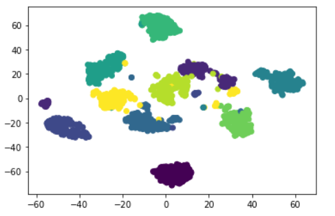

Scatterplot

In conclusion, PCA and t-SNE are two popular dimensionality reduction techniques that can be used to simplify large amounts of data. With the help of Python libraries like scikit-learn and matplotlib, these techniques can be easily implemented and their results visualized.

Before you go

I hope you enjoyed reading this article and find it useful. Please consider following me on | GitHub | Linkedin | Kaggle |

Vishnu Viswanath